As a reminder, entropy represents the level of uncertainty/randomness in the data or unpredictability associated with a random variable drawn from some distribution. That is, it shows how mixed or varied the data is, high entropy values means high uncertainty and very hard to predict, while low entropy means low uncertainty. Mathematically information entropy is calculated as:
H(X)=−i=1∑npilog2(pi)(1)where n is the number of classes, and pi is the probability of class i.
The uniform distribution has the highest entropy since all outcomes are equally likely, in this case, the entropy is:
H(X)=−i=1∑nn1log2(n1)(2) =log2(n)Lets go through an example to solidify the concept. Let's assume we had a hypothetical country of 6 people from 2 tribes. Without any split, the entropy would be:
−(63log2(63)+63log2(63))=1 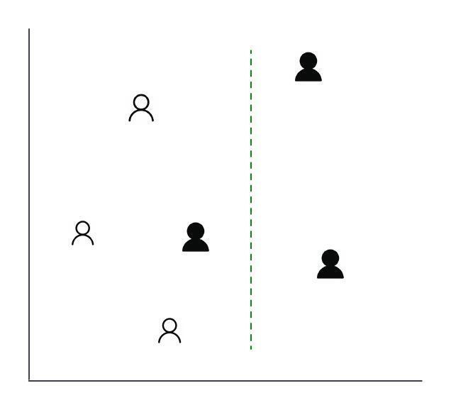
Updated : Jan 9 2025 - Thanks to a kind reader for pointing out an error in the previous image.
However, with that split, the right side after the split with two people would have entropy of 0, and left side would have entropy of :
−(41log2(41)+43log2(43))≈0.811The weighted entropy for both sides would be:
(62×0)+(64×0.811)≈0.541 =1−0.541≈0.459Cross-entropy extends the idea of entropy when there exists two distributions (actual observed distribution and predicted data distribution). It is mostly useful in tracking the training loss of classification ML models. Mathematically, if the actual is (P) and predicted (Q), then each cross-entropy:
Hce(P,Q)=−i=1∑nPilog2Qi(3)With our six people example in the previous section, let's assume we had a road and some ML algorithm to predict who has pass the road among the six people. Hence assuming the two probability distributions for each road:
Actual probabilities (P)0.30.20.150.150.10.1Predicted probabilities (Q)0.10.050.150.20.250.25The cross-entropy for the two distribution would be:
Hce(P,Q)=−(0.3log20.1+0.2log20.05+0.15log20.15+0.15log20.2+0.1log20.25+0.1log20.25) ≈3.26However if the probability distribution between the Actual and predicted were similar as:
Actual probabilities (P)0.30.20.150.150.10.1Predicted probabilities (Q)0.280.220.140.160.110.09The cross-entropy would be:
Hce(P,Q)=−(0.3log20.28+0.2log20.22+0.15log20.14+0.15log20.16+0.1log20.11+0.1log20.09) ≈2.38Consider selecting a number in the of range of 1 to 12 n∈{1,…,12}. Let X(n) be 1 if n is even, and Y(n) be 1 if n is divisible by 3.
NumberXY100210301410500611700810901101011001211Since (X=0,Y=0) occurs at n∈{1,5,7,11}, (X=0,Y=1) occurs at n∈{3,6}, (X=1,Y=0) occurs at n∈{2,4,8,10}, and (X=1,Y=1) occurs at n∈{6,12}. We can summarize the joint distribution of X and Y as:
P(X,Y)X=0X=1Y=0124124Y=1122122And our joint entropy would be:
=−(124log2124+122log2122+124log2124+122log2122) ≈1.918Joint entropy is a measure of the total uncertainty associated with a set of random variables.Therefore we can represent it a formula as used above is:
H(X,Y)=−x∈X∑y∈Y∑P(x,y)log2P(x,y)(4)OR
H(X,Y)=−x,y∑P(x,y)log2P(x,y)(5)This is a measure of predictability. The lowest perplexity is 1, which means the outcome is certain. Higher perplexity values indicate more uncertainty. It is calculated as:
Perplexity(P)=2Hce(P)(6)KL divergence is an extension of cross-entropy for statistical comparison of two probability distributions. It solves the inherent uncertainity problem in cross-entropy since H(P,P)=H(P). This is because cross-entropy satisfies H(P,Q)=H(P)+DKL(P∣∣Q)andH(P,P)=H(P)>0 in general, it does not vanish even when (Q=P). Hence KL divergence subtracts the entropy of the actual distribution from the cross-entropy resulting in:
DKL(P,Q)=Hce(P,Q)−H(P)(7) =−(j=1∑npjlog2qj−j=1∑npjlog2pj)(8)Mutual information is very similar to KL divergence; the main difference is that while KL divergence compares how similar two distributions are, mutual information measures the dependency between two random variables by calculating the KL divergence between their joint distribution P(X,Y) and the product of their marginals P(X)P(Y) which is calculated as:
I(X;Y)=x∈X∑y∈Y∑p(x,y)log(p(x)p(y)p(x,y))(9)With another representation as:
I(X;Y)=H(X,Y)−H(X/Y)−H(Y/X)(10) =H(X)+H(Y)−H(X,Y)(11)Reconsider the joint entropy example above with X and Y. First the conditional distributions P(Y/X) normalizing each row:
P(Y/X)X=0X=1Y=06/124/12=326/124/12=32Y=16/122/12=316/122/12=31Then calculating the conditional entropy H(Y/X):
=−(32log232+31log231+32log232+31log231) ≈0.918Hence the mutual information between X and Y would be:
I(X;Y)=H(X)−H(Y/X) =1−0.918 =0.082And we can verify joint entropy with the mutual information formula as:
H(X,Y)=H(X)+H(Y)−I(X;Y)(12) =1+1−0.082=1.918Understanding these concepts is crucial since all the machine learning algorithms are based on the idea of minimizing some form of a loss function which is often a variation of the above concepts.